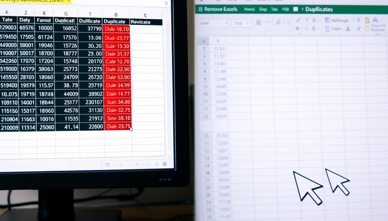
Duplicate data in Excel can slow down analysis, lead to errors, and waste time. Whether you are cleaning a mailing list, reconciling transactions, or preparing a report, knowing how to remove duplicates accurately is essential. Excel offers multiple ways to handle duplicate values, from a dedicated button and keyboard shortcuts to formulas and Power Query. Each method suits different scenarios, and choosing the right one depends on your dataset, whether you need to keep the first instance, and if the cleanup is one‑time or recurring.
This article covers the fastest shortcut, the safest way to keep one record, formula‑based detection, non‑destructive identification, and handling multiple columns. All instructions are based on Excel 2016 and later versions unless noted.
How to Remove Duplicates in Excel: The Fastest Shortcut Method
Best for: Quick, single or multi‑column removal
Steps: Data tab → Remove Duplicates
Time: ~30 seconds
Best for: Power users avoiding mouse
Steps: Alt + A + M
Time: ~5 seconds
Best for: Dynamic, repeatable duplicate detection
Steps: =COUNTIF(range, criteria)
Time: ~2 minutes
Best for: Identifying before deleting
Steps: Home → Conditional Formatting → Duplicate Values
Time: ~20 seconds
- The ‘Remove Duplicates’ button in the Data tab is the fastest method for most users, supporting both single and multiple columns.
- There is no single dedicated ‘remove duplicates’ shortcut key, but Alt + A + M is the fastest keyboard sequence (Excel 2016+).
- To keep the first instance and delete subsequent duplicates, use the built‑in Remove Duplicates button – it always keeps the first occurrence by default.
- For dynamic analysis, formulas like COUNTIF or UNIQUE (Excel 365) allow duplicate identification without altering original data.
- Conditional Formatting is the best non‑destructive method for visually identifying duplicates before taking action.
| Feature | Location / Example | Supports Multiple Columns | Keeps First Instance |
|---|---|---|---|
| Built‑in Button | Data → Data Tools → Remove Duplicates | Yes | Yes |
| Keyboard Shortcut | Alt + A + M | Yes | Yes |
| Formula (COUNTIF) | =COUNTIF(A:A, A2)>1 | No (single column per formula) | Yes (with filter) |
| Conditional Formatting | Home → Conditional Formatting → Duplicate Values | Yes (applied to range) | N/A (visual only) |
| UNIQUE Function | =UNIQUE(A2:A100) | Yes (with array context) | Yes (returns distinct values) |
| Advanced Filter | Data → Sort & Filter → Advanced → Unique records only | Yes | Yes |
| Power Query | Data → From Table/Range → Remove Duplicates | Yes | Yes |
How to Delete Duplicates in Excel but Keep One (or the First Instance)
The built‑in Remove Duplicates tool naturally retains the first record it encounters. The “first” row is determined by the current order of your data. If you need a different record to survive – for example, the most recent transaction – sort the data before removing duplicates.
Sorting before removal
Before clicking Remove Duplicates, sort your data so the record you want to keep appears first. For instance, sort by date descending to keep the newest entry, then apply the removal.
Always sort your data on the field that defines which instance is “best” (e.g., highest priority, latest date) before using Remove Duplicates. The tool keeps the first row in the sorted order.
Using Power Query for repeatable workflows
For recurring reports where you must always keep the first instance after a specific sort, Power Query offers a reusable solution. Load your table into Power Query, apply the sort, remove duplicates, and load the result back to Excel. The same steps can be refreshed whenever the source data changes.
How to Remove Duplicates in Excel Using a Formula
Formulas give you control without permanently changing your data. The COUNTIF function is the most common way to flag duplicates. In a helper column, enter =COUNTIF($A$1:A2, A2) and copy down. A result of 1 means the value is appearing for the first time; anything greater indicates a duplicate.
Filtering duplicates after flagging
Once the helper column is in place, you can filter for values greater than 1 and delete those rows. This gives you a clear audit trail before any removal.
The UNIQUE function (Excel 365)
Excel 365 subscribers can use =UNIQUE(range) to return a dynamic list of distinct values. This does not modify the original data and updates automatically when the source changes. It is ideal for extracting a clean list without deleting anything.
The COUNTIF approach works on single columns per formula. For multiple‑column duplicate detection, you will need a combined helper column (e.g., concatenating first name and last name) or use the built‑in button. The UNIQUE function is only available in Excel 365 and Excel for the web.
How to Identify or Highlight Duplicates in Excel Without Deleting Them
Before removing any data, you may want to review duplicates visually. Conditional Formatting is the fastest way to highlight duplicate values.
Using Conditional Formatting
Select your data range, go to Home → Conditional Formatting → Highlight Cells Rules → Duplicate Values, and choose a formatting style. All duplicate cells will be highlighted instantly. This method is non‑destructive and works on single or multiple columns.
Using COUNTIF for advanced review
A helper formula with COUNTIF gives you more flexibility. For example, =COUNTIF($A$2:$A$100, A2)>1 returns TRUE for duplicates. You can then apply a custom conditional formatting rule based on this formula to highlight only certain types of duplicates.
Conditional formatting and the Remove Duplicates button may behave unpredictably on ranges that contain merged cells. It is best to unmerge cells before running any duplicate detection.
How to Remove Duplicates in Excel Based on Multiple Columns
When duplicates are defined by more than one column – for example, the same First Name and Last Name – you need to tell Excel which columns to compare.
Using the Remove Duplicates button with multiple columns
Click Data → Remove Duplicates. In the dialog, uncheck all columns except the ones that define a duplicate. Excel will remove rows where the values in those selected columns are identical. The first occurrence is kept.
Using Power Query for multi‑column duplicates
Power Query works similarly: after loading your data, select the columns to compare (hold Ctrl to choose multiple), then right‑click and select Remove Duplicates. This method is especially useful for large datasets that need repeated cleaning.
How Has Excel’s Duplicate Removal Evolved Over Time?
- – Excel 2007 introduces the ‘Remove Duplicates’ button in the Data tab.
- – Power Query add‑in introduced, bringing advanced duplicate handling.
- – Remove Duplicates becomes standard; the keyboard shortcut Alt+A+M is widely adopted.
- – Excel 365 adds the UNIQUE formula for dynamic duplicate removal.
- – Current best practice: use Remove Duplicates for one‑time cleanup, Power Query for recurring workflows, and formulas for dynamic detection.
What Do We Know for Certain About Removing Duplicates? What Remains Unclear?
| Established Information | Information That Remains Unclear |
|---|---|
| Remove Duplicates button always keeps the first occurrence. | Whether the user has Excel 365 (UNIQUE formula) vs an older version. |
| Alt + A + M works in Excel 2016 and later versions. | Exact behavior with merged cells – can cause unexpected results. |
| COUNTIF formula identifies duplicates reliably. | Whether “duplicate” is defined by entire row vs selected columns – user must specify. |
| Multiple columns can be selected in the Remove Duplicates dialog. | – |
Choosing the Right Method for Your Data
For a one‑time cleanup on a static dataset, the Remove Duplicates button is fastest and most reliable. For ongoing reports, use Power Query to automate duplicate removal as data refreshes. For auditing and review, use Conditional Formatting or COUNTIF to see duplicates before deleting. For large datasets (10,000+ rows), the built‑in button is still efficient, but Power Query may be faster for repeated operations. Always back up your data before using Remove Duplicates, as the action is irreversible in the same session.
What Do Official Sources and Experts Say?
“Select the range of cells that has duplicate values, then click Data > Remove Duplicates.”
– Microsoft Support
Community experts at Excel Campus also recommend sorting data before removing duplicates to ensure the desired record is kept. While Microsoft’s official documentation covers the button method thoroughly, formula‑based and Power Query approaches are less prominent there, yet widely taught by Excel trainers.
Which Method Suits Your Workflow Best?
The best method depends on how frequently you clean data and whether you need to preserve the original dataset. For quick, one-time removal, the Remove Duplicates button or the Alt + A + M shortcut is ideal. For repeatable processes, Power Query saves time. For live lists that must update automatically, the UNIQUE function is the modern choice. No matter which method you pick, always back up your data first.
Frequently Asked Questions
How to remove duplicates in Excel without formula?
Use the built‑in ‘Remove Duplicates’ button under the Data tab, or use Conditional Formatting to highlight and then manually delete.
How to find duplicate values in Excel using formula?
Use =COUNTIF(A:A, A2)>1 in a helper column. If the result is TRUE, the value appears more than once.
How to identify duplicates in Excel without deleting?
Use Conditional Formatting (Home → Conditional Formatting → Highlight Cells Rules → Duplicate Values) to visually mark duplicates.
How to highlight duplicates in Excel?
Select your data range, go to Home → Conditional Formatting → Highlight Cells Rules → Duplicate Values, then choose a format.